6 Simple Techniques For Excel If Function

The feature informs the spreadsheet the kind of formula. If a math function is being executed, the mathematics formula is surrounded in parentheses. Utilizing the range of cells for a formula. As an example, A 1: A 10 is cells A 1 through A 10. Formulas are developed making use of absolute cell recommendation.

In our first formula participated in the cell "D 1," we by hand get in a =sum formula to add 1 +2 (in cells A 1 and B 2) to obtain the overall of "3." With the following instance, we utilize the highlight cells A 2 to D 2 and also after that rather than typing the formula utilize the formula switch in Excel to instantly produce the formula.

Ultimately, we manually get in a times (*) formula utilizing sum function to discover the value of 5 * 100. Note The features listed here might not be the exact same in all languages of Microsoft Excel. All these examples are done in the English variation of Microsoft Excel. Tip The examples listed below are noted in indexed order, if you wish to start with one of the most common formula, we recommend starting with the =SUM formula.

=STANDARD(X: X) Present the ordinary quantity between cells. For example, if you wished to obtain the standard for cells A 1 to A 30, you would type: =STANDARD(A 1: A 30). =MATTER(X: X) =COUNTA(X: X) Count the variety of cells in an array which contain any type of message (message and also numbers, not only numbers) and are not empty.

The 45-Second Trick For Excel If Statement

If 7 cells were vacant, the number "13" would be returned. =COUNTIF(X: X,"*") Count the cells that have a specific value. For instance, if you have =COUNTIF(A 1: A 10,"EXAMINATION") in cell A 11, after that any type of cell between A 1 through A 10 that has words "test" will certainly be counted as one.

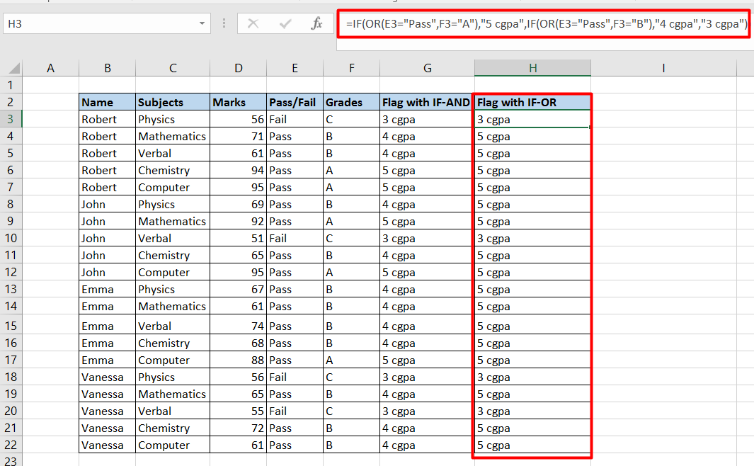
For example, the formula =IF(A 1="","SPACE","NOT SPACE") makes any cell besides A 1 state "BLANK" if A 1 had nothing within it. If A 1 is not empty, the various other cells will certainly read "NOT BLANK". The IF statement has much more intricate uses, but can normally be minimized to the above framework.

As an example, you might be splitting the values between 2 cells. Nevertheless, if there is nothing in the cells you would certainly obtain the =INDIRECT("A"&"2") Returns a reference specified by a text string. In the above example, the formula would return the value of the cell consisted of in A 2.

=TYPICAL(A 1: A 7) Discover the average of the values of cells A 1 with A 7. As an example, four is the mean for 1, 2, 3, 4, 5, 6, 7. =MIN/MAX(X: X) Minutes and also Max represent the minimum or optimum amount in the cells. For instance, if you desired to obtain the minimum value in between cells A 1 and also A 30 you would certainly place =MINUTES(A 1: A 30) or if you wished to get the optimum about =MAX(A 1: A 30).

The Buzz on Excel If Formula

For example, =Item(A 1: A 30) would numerous all cells together, so A 1 * A 2 * A 3, and so on =RAND() Generates a random number more than absolutely no but much less than one. For instance, "0.681359187" might be a randomly created number placed into the cell of the formula. =RANDBETWEEN(1,100) Create a random number in between two values.

=ROUND(X, Y) Round a number to a particular number of decimal locations. X is the Excel cell including the number to be rounded. Y is the variety of decimal locations to round. Below are some instances. =ROUND(A 2,2) Beats the number in cell A 2 to one decimal place. If the number is 4.7369, the above instance would round that number to 4.74.

=ROUND(A 2,0) Rounds the number in cell A 2 to absolutely no decimal places, or the nearest whole number. If the number is 4.736, the above instance would certainly round that number to 5. If the number is 4.367, it would round to 4. =AMOUNT(X: X) One of the most typically utilized feature to add, deduct, numerous, or divide worths in cells.

=SUM(A 1+A 2) Add the cells A 1 and A 2. =AMOUNT(A 1: A 5) Include cells A 1 with A 5. =AMOUNT(A 1, A 2, A 5) Includes cells A 1, A 2, and A 5. =SUM(A 2-A 1) Subtract cell A 1 from A 2. =AMOUNT(A 1 * A 2) Multiply cells A 1 as well as A 2.

Excel If for Dummies

=SUMIF(X: X,"*"X: X) Carry out the SUM function just if there is a specified worth in the initial chosen cells. An example of this would certainly be =SUMIF(A 1: A 6,"EXAMINATION", B 1: B 6) which only adds the values B 1: B 6 if words "test" was placed somewhere in between A 1: A 6. So if you put EXAMINATION (not situation sensitive) in A 1, yet had numbers in B 1 with B 6, it would only include the worth in B 1 due to the fact that TEST remains in A 1.

=TODAY() Would certainly print out the existing date in the cell gotten in. The value will certainly change each time you open your spreadsheet, to show the existing day and time. If you intend to enter a day that does not change, hold down semicolon) to go into the date. =FAD(X: X) To discover the common value of cell.

=VLOOKUP(X, X: X, X, X) The lookup, hlookup, or vlookup formula enables you to browse and also locate relevant worths for returned outcomes. See our lookup interpretation for a full interpretation and complete details on this formula. .

Each IF feature in an Excel spread sheet returns one of two messages. The very first-- the "if" message-- displays if cells meet standards that you define. The second-- the "or else" message-- displays if they do not. As an example, mean that your sheet tracks the hours that each of your staff members works.

excel if formula symbols excel if formula match excel if formula else